Neural Networks CheatSheet

DNN

For the forward and backward pass of fully connected layer, rules are quite simple:

$$ \begin{eqnarray*} Y &=& A \cdot B \rightarrow dA = dY \cdot B^T, dB=A^T \cdot dY \\ Y&=&A^T \cdot B \rightarrow dA=(dY \cdot B^T)^T=B \cdot dY^T, dB=A^T \cdot dY \\ Y&=&A \cdot B^T \rightarrow dA=dY \cdot B^T, dB=(A^T \cdot dY)^T=dY^T \cdot A \\ Y&=&A^T \cdot B^T \rightarrow dA=(dY \cdot B^T)^T=B \cdot dY^T, dB=(A^T \cdot dY)^T=dY^T \cdot A \end{eqnarray*} $$

CNN

Conv Forward

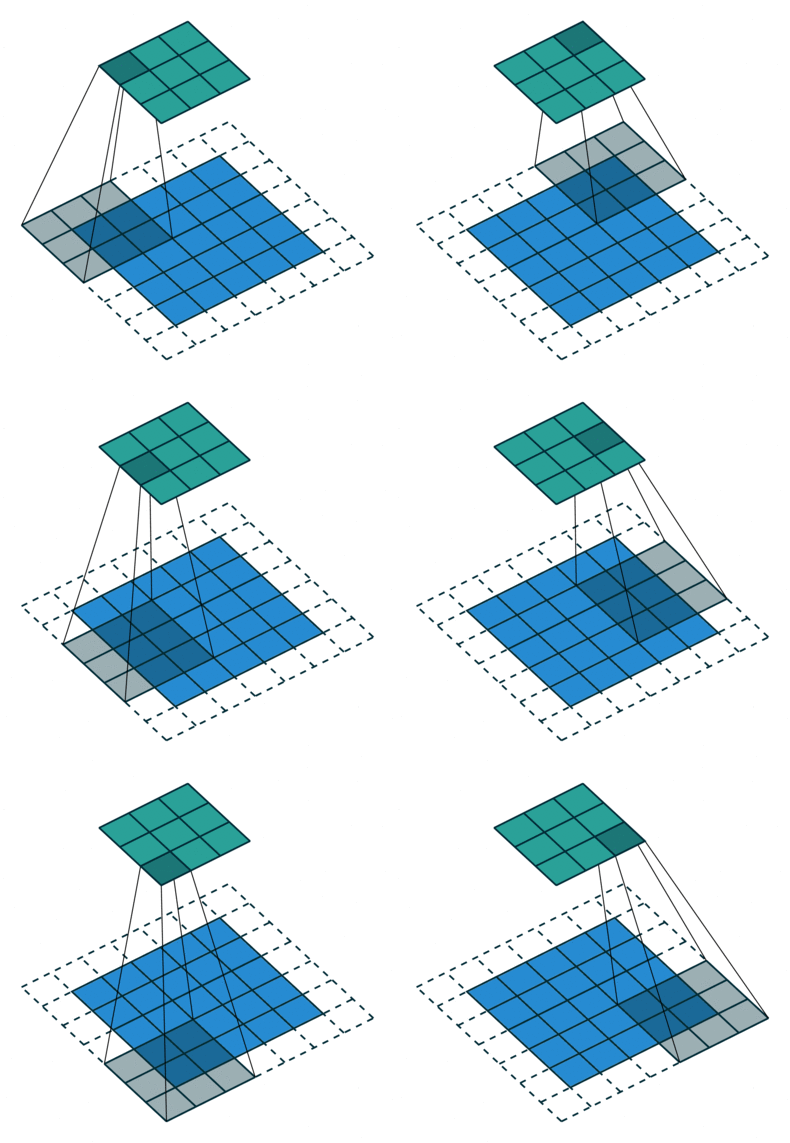
Here is a convolution example with $i=5,k=3,s=2,p=1$:

CONV

im2col

Given input Tensors of image $I^{i_c,i_h,i_w}$ with channels $i_c$, height $i_h$ and width $i_w$; kernel $K^{o_c,i_c,k_h,k_w}$ with output channels (also # of kernels) $o_c$, input channels $i_c$, kernel height $k_h$ and width $k_w$, we hope to compute is convolution result $O^{o_c,o_h,o_w}$.

With im2col we expand $I^{i_c,i_h,i_w}$ into a larger Matrix: $I^{i_c k_h k_w, o_h o_w}$, then we do GEMM:

$$ K^{o_c,i_c k_h k_w} \cdot I^{i_c k_h k_w, o_h o_w} \rightarrow O^{o_c,o_h o_w} $$

Each column of this expanded matrix $I^{i_c k_h k_w, o_h o_w}$ has same size with a kernel ($i_c k_h k_w$), and size of each row equals to the size of a single channel ($o_h o_w$) in output image. The image is expanded in a specific way to guarantee that when doing matmul, the accumulation of this row*column is exactly same as doing convolution.

Conv Backward

Consider a simple case of 3x3 kernel with n channels.

$$ \begin{eqnarray*} z^{l+1}_{c,i,j}=\sum_{c=1}^{n}&(&a^l_{c,i-1,j-1}k_{c,1,1}&+&a^l_{c,i-1,j}k_{c,1,2}&+&a^l_{c,i-1,j+1}k_{c,1,3} \\ &+&a^l_{c,i,j-1}k_{c,2,1}&+&a^l_{c,i,j}k_{c,2,2}&+&a^l_{c,i,j+1}k_{c,2,3} \\ &+&a^l_{c,i+1,j-1}k_{c,3,1}&+&a^l_{c,i+1,j}k_{c,3,2}&+&a^l_{c,i+1,j+1}k_{c,3,3} ) \end{eqnarray*} $$

$$ a^{l+1}_{i,j}=f(z^{l+1}_{i,j}) $$

$$ \delta^{l+1}_{c,i,j}=\frac{\partial L}{\partial a^{l+1}_{c,i,j}} $$

The value of $a^{l}_{c,i,j}$ affects $3*3=9$ values in $a^{l+1}$. Thus, to compute gradient w.r.t to the image input, we can just rotate the convolution kernel for 180 degrees and do convolution again.

For non-unit stride, things become more complicated. The backward procedure of convolution is still doing convolution with rotated kernels on gradients of output feature maps, but before we do that, the gradients should be not only padded with $p^{'}$, but also dilated with size $s - 1$. Finally, the backward process should still be done with stride $s^{'}=1$.

Consider the 2-D simple case without image channels, the size of output feature map should be:

$$ o = \frac{i - k + 2p}{s} + 1 $$

Thus we have inverse form:

$$ i = s(o - 1) - 2p + k $$

Since we know the output feature map should be dilated with size $s - 1$, then it should have new size $s(o - 1) + 1$. So we will have:

$$ s(o - 1) + 1 - k + 2 * p^{'} + 1 = s(o - 1) - 2p + k $$

Finally we got $p^{'} = k - p - 1$. This is the padding we used on back propagation of gradients. For the example convolution above, the corresponding backward procedure is shown below with $s^{'}=1,p^{'}=3-1-1=1$.

DCONV

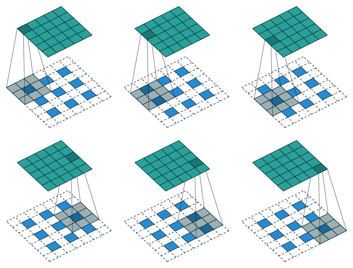
As for the gradients of filter, things would be quite similar. We just use the gradients of output feature maps as kernels, to do convolution on input images. Before using as kernels, the gradients should also be dilated with size $s-1$.

In this way, we're doing a convolution with new kernel $k^{'}=s(o-1)+1$, new stride $s^{'}=1$, we need to know its new padding. Thus we have:

$i - (s(o-1)+1) + 2p^{'} + 1 = k$

Recall that $i = s(o - 1) - 2p + k$, we will get $p^{'}=p$, which means we only need to use same padding as forward convolution.

There is also a subtle difference on gradients computation of filters. Suppose the input images have $C_{in}$ channels, and output images have $C_{out}$ channels, which also means we have $C_{out}$ filters. Each time we take channel $c$ of $C_{out}$ channels in the output feature maps (actually gradients), use it as a kernel to do convolution on different channels of input images for $C_{in}$ times, and we will get gradients of the $c$-th kernel with size $[C_{in}, k, k]$. This procedure will be executed for $C_{out}$ times, and finally we'll get gradients for all $C_{out}$ kernels.

col2im

For im2col implementation, suppose we have back-propagated gradient Tensor $G_l^{o_c, o_h, o_w}$ from next layer, which should have same size with convolution output. The backward phase would be:

$$ (K^{o_c,i_c k_h k_w})^T \cdot G_l^{o_c, o_h o_w} \rightarrow dI^{i_c k_h k_w, o_h o_w} \\ G^{o_c, o_h o_w} \cdot (I^{i_c k_h k_w, o_h o_w})^T \rightarrow dK^{o_c, i_c k_h k_w} $$

Then we could use a col2im function to aggregate gradients in $dI^{i_c k_h k_w, o_h o_w}$ into actual gradient Tensor $G_{l-1}^{i_c,i_h,i_w}$ as gradient input to previous layer.

Notice that we don't have to do real transpose in actual implementation. Also keep in mind that for batch_size > 1, we should aggregate all the computed gradient of images in this batch.

Word Embedding

Basic Concepts

Common Ways to Represent Words:

One-Hot vectors:
The vector length equals the size of the vocabulary. One element in the vector is set to 1, while all others are 0, thereby uniquely representing a word.
Word Embedding:
Word embeddings map ultra–high-dimensional one-hot vectors (with dimensionality depending on the vocabulary size, potentially reaching hundreds of thousands) into floating-point vectors of a few hundred dimensions. Mathematically, this is referred to as an embedding.
Their key property is that they preserve semantic information: words with similar meanings are closer to each other (i.e., have smaller angles or distances between their vectors). Well-trained word embeddings can also capture relational structure, such as the distance between Beijing and China being approximately equal to the distance between London and the United Kingdom (but how can deeper, multi-level semantic relationships be represented?).

How to Handle Polysemous Words:

Word vectors are typically learned jointly with model training—that is, they are obtained as part of training a target model.

Language Model

Given word sequence $w_1, w_2, ..., w_t$, we hope to know the probability of whether it is a natural language sequence or not, which is defined as $P(w_1, w_2, …, w_t)$, thus we have:

$$ P(w_1, w_2, …, w_t) = P(w_1) \times P(w_2 | w_1) \times P(w_3 | w_1, w_2) \times … \times P(w_t | w_1, w_2, …, w_{t-1}) $$

As for simple N-gram model, $P(w_t | w_{t-n+1}, …, w_{t-1})$ is a good approximation.

RNNLM

LSTM

Given a time series of data vectors and their corresponding output labels (also could be vectors), we hope to train the LSTM network such that at each time step we input a single vector, the network could give us an output very close to its corresponding label, which is measured by predefined loss function.

Forward Pass

The forward pass of an LSTM step is defined as follows according to this article:

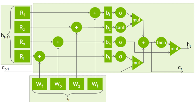
$$ \begin{eqnarray} g(t) &=& \phi(W_{gx} x(t) + W_{gh} h(t-1) + b_{g}) \\ i(t) &=& \sigma(W_{ix} x(t) + W_{ih} h(t-1) + b_{i}) \\ f(t) &=& \sigma(W_{fx} x(t) + W_{fh} h(t-1) + b_{f}) \\ o(t) &=& \sigma(W_{ox} x(t) + W_{oh} h(t-1) + b_{o}) \\ s(t) &=& g(t) * i(t) + s(t-1) * f(t) \\ h(t) &=& s(t) * o(t) \\ \end{eqnarray} $$

LSTM Arch

With $x_c(t) = [x(t), h(t-1)]$, above (1) ~ (4) could be simplified to:

$$ \begin{eqnarray*} g(t) &=& \phi(W_{g} x_c(t) + b_{g}) \\ i(t) &=& \sigma(W_{i} x_c(t) + b_{i}) \\ f(t) &=& \sigma(W_{f} x_c(t) + b_{f}) \\ o(t) &=& \sigma(W_{o} x_c(t) + b_{o}) \end{eqnarray*} $$

Notice that all these six states $g, i, f, o, s, h$ above could be represented as a vector of same length, which is just the length of memory cells.

Back prorogation through time

Suppose we have a loss $l(t)$ that we wish to minimize at every time step $t$ that depends on the last hidden layer $h$ and the expected label $y$ at the current time step via a loss function $f$:

$$l(t) = f(h(t), y(t))$$

Where $f$ can be any differentiable loss function, such as the Euclidean loss:

$$l(t) = f(h(t), y(t)) = \| h(t) - y(t) \|^2$$

Our ultimate goal in this case is to use gradient descent to minimize the loss $L$ over an entire sequence of length $T$:

$$L = \sum_{t=1}^{T} l(t)$$

For gradient descent, what we care is the partial derivative of loss $L$ to each weight scalar $w$ in all those weight matrices listed above. After we got that, gradient descent could be applied as:

$$ w = w - \alpha * \frac{\partial L}{\partial w} $$

where $\alpha$ is our learning rate.

As label $y(t)$ is constant, this lost value $L$ depends directly on every scalar in the last hidden layer $h$ at every time step, which would be:

$$\frac{ \partial L}{ \partial w} = \sum_{t = 1}^{T} \sum_{i = 1}^{M} \frac{ \partial L}{ \partial h_i(t)}\frac{ \partial h_i(t)}{ \partial w}$$

where $h_i(t)$ is the scalar corresponding to the $i$’th memory cell in the hidden output vector, and $M$ is the length of hidden output vector.

Since the network propagates information forwards in time, changing $h_i(t)$ will have no effect on the loss values $l(s)$ earlier than time step $t$, which means:

$$ \sum_{s=1}^{t-1} \frac{\partial l(s)}{\partial h_i(t)} = 0 $$

Thus we've got:

$$ \begin{eqnarray*} \frac{ \partial L}{ \partial h_i(t)} &=& \sum_{s=1}^T \frac{ \partial l(s)}{ \partial h_i(t)} = \sum_{s=t}^T \frac{ \partial l(s)}{ \partial h_i(t)} \end{eqnarray*} $$

For notational convenience, we introduce the variable $L(t)$ that represents the cumulative loss from time step $t$ to the end state $T$:

$$ L(t) = \sum_{s=t}^{T} l(s) $$

such that $L(1)$ is the loss for the entire sequence. This allows us to rewrite the above equation as:

$$ \frac{\partial L}{\partial h_i(t)} = \sum_{s=t}^T \frac{\partial l(s)}{\partial h_i(t)} = \frac{\partial L(t)}{\partial h_i(t)} $$

With this in mind, we can re-write our gradient calculation as:

$$ \frac{\partial L}{\partial w} = \sum_{t = 1}^{T} \sum_{i = 1}^{M} \frac{\partial L(t)}{\partial h_i(t)}\frac{\partial h_i(t)}{\partial w} $$

It is easy to calculate $\frac{\partial h_i(t)}{\partial w}$ according to forward propagation equations listed above. We now need to compute $\frac{\partial L(t)}{\partial h_i(t)}$, which is simplified to $\frac{\partial L(t)}{\partial h(t)}$ in formulas listed below to get a cleaner notation. Just keep in mind that same derivation will apply for each element in hidden output vector $h(t)$.

According to definition of $L(t)$, we could express the following recursion:

$$ L(t) = \begin{cases} l(t) + L(t+1) & \text{if} \, t < T \\ l(t) & \text{if} \, t = T \end{cases} $$

Thus, given activation $h(t)$ of an LSTM node at time step $t < T$, we have:

$$ \frac{\partial L(t)}{\partial h(t)} = \frac{\partial l(t)}{\partial h(t)} + \frac{\partial L(t+1)}{\partial h(t)} $$

When we start from the end of time series by:

$$ \frac{\partial L(T)}{\partial h(T)} = \frac{\partial l(T)}{\partial h(T)} $$

and gradient $\frac{\partial L(t)}{\partial h(t)}$ on each time step $t$ could be calculated. This is where the so called "back propagation through time" algorithm show up.

We use $g_{in}(t), i_{in}(t), f_{in}(t), o_{in}(t)$ to represent inputs of all those cells listed in (1) ~ (4), which should be vectors of same length with the cell:

$$ \begin{eqnarray*} g_{in}(t) &=& W_{g} x_c(t) + b_{g} \\ i_{in}(t) &=& W_{i} x_c(t) + b_{i} \\ f_{in}(t) &=& W_{f} x_c(t) + b_{f} \\ o_{in}(t) &=& W_{o} x_c(t) + b_{o} \end{eqnarray*} $$

Obviously their gradients would be as follows:

$$ \begin{eqnarray*} \phi^{'}(x) = 1 - \phi (x)^2 \\ \sigma^{'}(x) = x(1 - \sigma (x)) \\ \end{eqnarray*} $$

$$ \begin{eqnarray*} \frac{\partial L(t)}{\partial g_{in}(t)}&=&\frac{\partial L(t)}{\partial s(t)}\frac{\partial s(t)}{\partial g(t)}\frac{\partial g(t)}{\partial g_{in}(t)} \\ &=& \frac{\partial L(t)}{\partial s(t)}\phi^{'}(g_{in}(t))i(t) \\ &=& \frac{\partial L(t)}{\partial s(t)}(1-g(t)^2)i(t) \\ \frac{\partial L(t)}{\partial i_{in}(t)}&=&\frac{\partial L(t)}{\partial s(t)}\frac{\partial s(t)}{\partial i(t)}\frac{\partial i(t)}{\partial i_{in}(t)} \\ &=& \frac{\partial L(t)}{\partial s(t)}i(t)(1-i(t))g(t) \\ \frac{\partial L(t)}{\partial f_{in}(t)}&=&\frac{\partial L(t)}{\partial s(t)}\frac{\partial s(t)}{\partial f(t)}\frac{\partial f(t)}{\partial f_{in}(t)} \\ &=& \frac{\partial L(t)}{\partial s(t)}f(t)(1-f(t))s(t-1) \\ \frac{\partial L(t)}{\partial o_{in}(t)}&=&\frac{\partial L(t)}{\partial h(t)}\frac{\partial h(t)}{\partial o(t)}\frac{\partial o(t)}{\partial o_{in}(t)} \\ &=& \frac{\partial L(t)}{\partial h(t)}o(t)(1-o(t))s(t) \end{eqnarray*} $$

In order to calculate gradients above, we also need $\frac{\partial L(t)}{\partial s(t)}$ at each time step $t$. Notice that $s(t)$ not only contributes to $h(t)$, but also contribute to $h(t+1)$ according to (5), so derivative $\frac{\partial L(t)}{\partial s(t)}$ should be as follows:

$$ \begin{eqnarray*} \frac{\partial L(t)}{\partial s(t)} &=& \frac{\partial L(t)}{\partial h(t)} \frac{\partial h(t)}{\partial s(t)} + \frac{\partial L(t)}{\partial h(t+1)} \frac{\partial h(t+1)}{\partial s(t)} \\ &=& \frac{\partial L(t)}{\partial h(t)} \frac{\partial h(t)}{\partial s(t)} + \frac{\partial L(t+1)}{\partial h(t+1)} \frac{\partial h(t+1)}{\partial s(t)} \\ &=& \frac{\partial L(t)}{\partial h(t)} \frac{\partial h(t)}{\partial s(t)} + \frac{\partial L(t+1)}{\partial s(t)} \\ &=& \frac{\partial L(t)}{\partial h(t)}o(t) + \frac{\partial L(t+1)}{\partial s(t)} \end{eqnarray*} $$

Thus, during the back-prop procedure in programming, we take gradient vectors $\frac{\partial L(t+1)}{\partial s(t)}$ and $\frac{\partial L(t)}{\partial h(t)}$ from upper layer, compute gradients for each cell, then compute $\frac{\partial L(t)}{\partial s(t-1)}$, $\frac{\partial L(t)}{\partial h(t-1)}$ and pass them down.

To compute $\frac{\partial L(t)}{\partial s(t-1)}$, we have:

$$ \frac{\partial L(t)}{\partial s(t-1)} = \frac{\partial L(t)}{\partial s(t)} \frac{\partial s(t)}{\partial s(t-1)}=\frac{\partial L(t)}{\partial s(t)}f(t) $$

Recall that $x_c(t) = [x(t), h(t-1)]$, thus to get $\frac{\partial L(t)}{\partial h(t-1)}$ we only need to compute $\frac{\partial L(t)}{\partial x_c(t)}$ as follows:

$$ \begin{eqnarray*} \frac{\partial L(t)}{\partial x_c(t)} &=& \frac{\partial L(t)}{\partial g_{in}(t)}\frac{\partial g_{in}(t)}{\partial x_c(t)} \\ &+& \frac{\partial L(t)}{\partial i_{in}(t)}\frac{\partial i_{in}(t)}{\partial x_c(t)} \\ &+& \frac{\partial L(t)}{\partial f_{in}(t)}\frac{\partial f_{in}(t)}{\partial x_c(t)} \\ &+& \frac{\partial L(t)}{\partial o_{in}(t)}\frac{\partial o_{in}(t)}{\partial x_c(t)} \end{eqnarray*} $$

In equations above it is easy to compute each element according to normal back propagation algorithm on weight multiplication.

At the last time step $t=T$, we have following boundary conditions:

$$ \begin{eqnarray*} \frac{\partial L(t+1)}{\partial s(t)}=0 \\ \frac{\partial L(t)}{\partial h(t)}=\frac{\partial l(t)}{\partial h(t)} \end{eqnarray*} $$

References

http://nicodjimenez.github.io/2014/08/08/lstm.html
http://deeplearning.net/software/theano/tutorial/conv_arithmetic.html