LSTM Forward Computation

Basic Operators

The computation formulas and derivatives of the LSTM model have already been summarized in Neural Networks CheatSheet. From the perspective of basic operators, it can be roughly described as shown below:

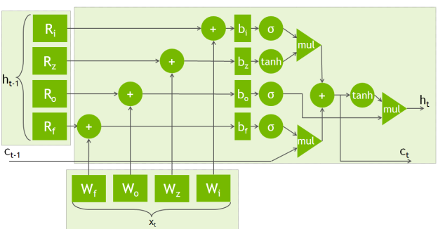
Considering computational parallelism, we can directly concatenate the four weight matrices into one large weight matrix. After multiplying it with \(x_t\), we Slice the result into four parts, which become the vector representations of the four Cells. Similarly, we can do the same weight merging for \(h_{t-1}\). After adding the two results and then applying Slice, the main computation of a basic Cell is completed. The subsequent operations are essentially corresponding Element-wise operations on the vectors of different Cells.

The computation process above is called a Node of the LSTM. If we look at the inputs and outputs of this Node, we can see that it takes a pair of states \([h_{t-1}, c_{t-1}]\) passed from the previous Node, as well as the current input vector \(x_t\), and then produces a pair of output states \([h_t, c_t]\). Among the output states, \(h_t\) is the actual output (vector) of the current Node, and it can also be denoted as \(y_t\); while \(c_t\) is output externally, so it does not affect the computation of the cost function, and is only passed as a hidden state to the next Node.

MXNet Implementation

For a process that takes inputs \(x_t\), \(h_{t-1}\), \(c_{t-1}\), performs a set of internal operations, and outputs \(h_t\), \(c_t\), its computation graph is actually easy to define. The MXNet implementation is as follows:

:::Python
def __call__(self, inputs, states):
    i2h = symbol.FullyConnected(data=inputs, weight=self._iW, bias=self._iB,
                                num_hidden=self._num_hidden*4,
                                name='%si2h'%name)
    h2h = symbol.FullyConnected(data=states[0], weight=self._hW, bias=self._hB,
                                num_hidden=self._num_hidden*4,
                                name='%sh2h'%name)
    gates = i2h + h2h
    slice_gates = symbol.SliceChannel(gates, num_outputs=4,
                                      name="%sslice"%name)
    in_gate = symbol.Activation(slice_gates[0], act_type="sigmoid",
                                name='%si'%name)
    forget_gate = symbol.Activation(slice_gates[1], act_type="sigmoid",
                                    name='%sf'%name)
    in_transform = symbol.Activation(slice_gates[2], act_type="tanh",
                                     name='%sc'%name)
    out_gate = symbol.Activation(slice_gates[3], act_type="sigmoid",
                                 name='%so'%name)
    next_c = symbol._internal._plus(forget_gate * states[1], in_gate * in_transform,
                                    name='%sstate'%name)
    next_h = symbol._internal._mul(out_gate, symbol.Activation(next_c, act_type="tanh"),
                                   name='%sout'%name)
    return next_h, [next_h, next_c]

As you can see, this is basically just translating the computation flow above into Python. One point to note is that the computation process above is in fact only an abstract computation defined on the computation graph: its effect is to build the corresponding graph structure, and it does not actually execute the computation. So where is the boundary between abstract computation and real computation? What kind of computation cannot be expressed as an abstract computation graph? My personal understanding is: as long as the computation does not depend on the actual values of the symbols, then this process can be described by a static computation graph. In the figure above, we know that when doing the Slice operation, we are going to split that vector into four parts, so this operation does not depend on the actual data values and can be described directly using nodes in the computation graph.

Static Computation Graph Implementation of LSTM

Loop Unroll

After implementing the computation of a single Node, as long as we are given the length of the input sequence \([x_1, x_2, ..., x_t]\), we can connect that many Node nodes end-to-end, so as to compute the corresponding output sequence \([y_1, y_2, ..., y_t]\). The unrolling of LSTM is roughly as shown below:

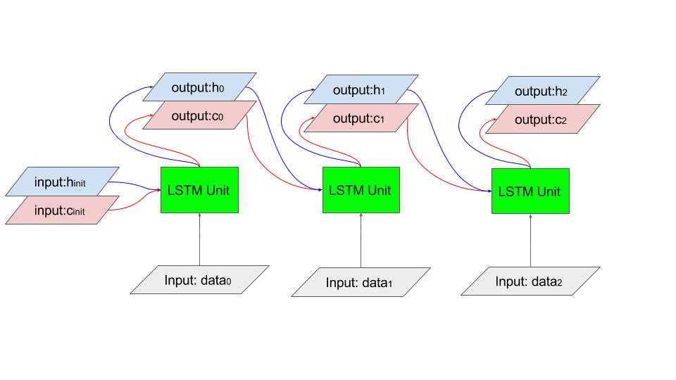
This process looks very simple: we only need to use the output of the previous node as the input to the next one, along with the corresponding data. Moreover, this is a general abstraction for RNN, so in MXNet it is implemented as a base-class method:

:::Python
def unroll(self, length, inputs, begin_state=None, layout='NTC', merge_outputs=None):
    self.reset()
    inputs, _ = _normalize_sequence(length, inputs, layout, False)
    if begin_state is None:
        begin_state = self.begin_state()
    states = begin_state
    outputs = []
    for i in range(length):
        output, states = self(inputs[i], states)
        outputs.append(output)
    outputs, _ = _normalize_sequence(length, outputs, layout, merge_outputs)
    return outputs, states

From the code above, we can see that we first need to obtain the initial input state (usually all zeros) to feed into the first Node. Then we can keep using the current Node's output as the next Node's input. This unrolling loop is straightforward. Also, in each iteration we must remember to save the current output, so that in the end we can compute the overall cost function and perform backpropagation. Overall, this part of the code is easy to understand.

After defining the LSTM in this unrolled way, it turns from a dynamic structure with a loop into a static computation graph structure. It is easy to imagine that at this point we no longer need the BPTT algorithm to train it. Because the computation graph is fixed and the computation process is finite, we can simply traverse it backward once according to the principle of automatic differentiation; the effect must be equivalent to BPTT.

Stack Multiple RNN Cells

Since the input of an RNN is a time series and its output is also a time series, an advanced approach is to stack multiple layers of Cells together—for example, stacking multiple layers of LSTM—to effectively improve the model's expressive power. Under a static computation graph framework, statically unrolling such a model is also very easy: we just need to iterate over all Cells, unroll them one by one, and use the output of the previous Cell as the input of the next Cell. In essence, it is the same as the unrolling of a single Cell.

The MXNet implementation is as follows:

:::Python
def unroll(self, length, inputs, begin_state=None, layout='NTC', merge_outputs=None):
    self.reset()
    num_cells = len(self._cells)
    if begin_state is None:
        begin_state = self.begin_state()
    p = 0
    next_states = []
    for i, cell in enumerate(self._cells):
        n = len(cell.state_info)
        states = begin_state[p:p+n]
        p += n
        inputs, states = cell.unroll(length, inputs=inputs, begin_state=states, layout=layout,
                                     merge_outputs=None if i < num_cells-1 else merge_outputs)
        next_states.extend(states)
    return inputs, next_states

You can see that this code structure is essentially not much different from unrolling a single Cell above, except that here we need to obtain the initial states for all Cells. One important difference is that only the output of the previous layer is connected to the input of the next layer, while the extra states of the previous layer's final output—such as \([h_t, c_t]\) in LSTM—are simply discarded. As an additional note, stacked RNNs work because the lower-layer network first performs feature extraction and transformation on the input sequence, and then feeds the resulting sequence into the next layer for processing, extracting higher-level features.

Sequence Buckets

After handling unrolling, we run into another problem: LSTM processes variable-length sequences, but once our static computation graph is defined, it can only handle fixed-length sequences. So the most brute-force solution is to create a static computation graph for every sequence length, and during training all subgraphs share weights—during backpropagation, we just update the same weight matrix. This is certainly feasible, but the resource consumption is excessive. A more reasonable approach is to first cluster all observed sequence lengths, find a few typical lengths, and then pad those uneven sequences to these lengths. Below is a quote from Yangqing Jia's description of this idea here:

A compromise solution is to first cluster sequences, preset a few fixed-length buckets, then put each sequence into its corresponding bucket and pad it to the fixed length. This way, first, we don't need to deal with a while loop: each bucket is a fixed computation graph; second, the padding for each sequence is small, so the waste of compute resources is limited; third, this is simple to implement: it's just length clustering, and it has low requirements on the framework.

Also, since we have padding, we naturally need special handling for the padding elements. In NLP, a common approach is to assign a special label such as -1 to padding elements, and then ignore this label when computing the loss.