[TVM Code Analysis] The NNVM Computation Graph Abstraction Mechanism

Hint: It is recommended to read this alongside the NNVM and TVM source code for the best flavor.

Design Overview

Graph Abstraction

In short, Symbol is used to abstract both Operator and Operand in a computation graph:

Variable Symbol
Functor Symbol (AtomicSymbol), callable semantics

More precisely, the abstraction Symbol represents a procedure with multiple inputs and outputs. A Symbol object contains only a single member vector<NodeEntry> outputs, used to record all of its output nodes in the graph; each Node, in contrast, records its own attributes and all input inputs. So the object that actually constructs the graph is Node: it can see all of its inputs; then the abstractions defined on top of the computation graph, such as Operand and Operator, are represented via Symbol.

In the graph representation, an Operator can compose some Operands into a new Operand, i.e., a node in the graph. In the end, we obtain a Symbol; from it we can trace back the entire graph and convert it into a Graph object to complete graph construction.

Different Operators have their own attributes. Common attribute definitions live in op_attr_types.h, basically various type declarations.

Core Data Structures

Node: Represents a node in IndexedGraph. Nodes are basically divided into Operator and Variable.
NodeEntry: Represents an input of some node in the graph. Therefore, for such an input, its data structure needs to record which node's output it belongs to, and which output index it is.

Python Interface

First, describe MXNet's definition of the basic elements of a computation graph. For a single Symbol and a composed Symbol (i.e., a Network), arguments are the data required to run the network forward, such as input data data and label, and layer weights such as Convolution's kernels, and Batch Norm's $\gamma$ and $\beta$. auxiliary_states refers to special states needed at runtime and worth persisting, such as Batch Norm's moving_mean and moving_var. In addition, inputs is the union of arguments and auxiliary_states. Finally, outputs naturally refers to the final outputs of the network; in most cases it is some form of Loss, but it may also be computed data, such as a GAN Generator.

The interface implementation in NNVM is very clean: the exported interfaces defined by the C API are few, and the Python code defines only the most core Symbol class, operator overloading, and necessary ctypes glue code. As for how to build graphs using Operators, that is registered into Python from C++ code via static definitions, and then dynamically registered into Python when import nnvm runs. The concrete implementation contains more details.

Implementation Details

Automatic Differentiation

Basic Principle

The principle of automatic differentiation is relatively straightforward; note that all variables are Tensors. Consider the basic property of an Operator: unlike a function, it maps multiple inputs to multiple outputs. So if the operator at the current node takes m inputs and returns n outputs, it can be formalized as:

$$Op(x_1, x_2, ..., x_m) = [f_1(x_1, ..., x_m), ..., f_n(x_1, ..., x_m)]$$

where $f_1, ..., f_n$ are the computation processes (functions) corresponding to different outputs.

Define a Gradient computation process for each operator. Its input is the derivative of the error $y$ with respect to all outputs of the current node (a list), and its output is the derivative of the error with respect to all inputs of the current node (also a list). The input can be formalized as $[\frac{\partial y}{\partial f_1(...)}, \frac{\partial y}{\partial f_2(...)}, ..., \frac{\partial y}{\partial f_n(...)}]$, then the output should be:

$$ [\sum_{i=1}^{n}\frac{\partial y}{\partial f_i}\frac{\partial f_i}{\partial x_1}, \sum_{i=1}^{n}\frac{\partial y}{\partial f_i}\frac{\partial f_i}{\partial x_2}, ..., \sum_{i=1}^{n}\frac{\partial y}{\partial f_i}\frac{\partial f_i}{\partial x_m}] $$

In addition, $\frac{\partial y}{\partial f_i(...)}$ is the accumulated result after summing over all partial-derivative paths from $y$ to an operator Op output $f_i(...)$. This implies all operators need to define an accumulation operation attribute; if not, MXNet will by default attempt to call __ewise_sum__ to accumulate. Note that all of the above computations are symbolic computations, not numeric computations, i.e., the computations produce new nodes on the graph.

Next, we traverse the network directly in reverse topological order. For the current node, we compute the aggregated result (a node) of the derivatives of all its outputs $[\frac{\partial y}{\partial f_i(...)}]$, then use the operator's Gradient method to compute derivatives w.r.t. all inputs $[\frac{\partial y}{\partial x_i}]$, and continue propagating backward. Reverse topological order ensures that when we reach the current node, all of its output nodes—i.e., all input nodes for backprop—have already finished differentiation.

In neural networks, gradient descent needs the derivative of the error $y$ w.r.t. the weight matrix $W$, so in automatic differentiation we only need to output the derivative nodes for those weight nodes we care about. In fact, if we know which nodes are weights, we can have the autodiff engine generate their derivative nodes. Then during training, assign storage for these gradient terms, so after one traversal of the computation graph, we can directly extract the gradients we want and update them.

MXNet Implementation Details

The figure below shows the Forward computation graph for a simple two-layer MLP:

MLP Forward

Then the backward differentiation process looks like this:

Compute the derivatives of softmax w.r.t. fc3 and softmax_label: softmax_backward.
At this point, we know the derivatives of $y$ w.r.t. all outputs of the fc3 node are [softmax_backward], so we can compute the derivatives of $y$ w.r.t. all inputs of fc3: [relu2, fc3_weight, fc3_bias].
And so on, completing the differentiation process in reverse topological order...

MLP Gradient

Here we notice that softmax has two input nodes with clearly different shapes, but only one derivative node softmax_backward; similarly, fc3 has three different inputs but also only one derivative node fc3_backward, and other nodes are similar. This is actually a historical artifact of MXNet's computation graph redesign. Because most old operators were not implemented according to the design described above—they do not include a Gradient method that can directly compute derivative nodes symbolically from node inputs. So for compatibility, when registering operators, MXNet registers backward operators with a _backward_ prefix for these legacy operators in NNVM. When differentiating the computation graph, it directly generates a node whose Operator is the _backward_ version, and lets the operator declare the data it depends on during backprop. Then when the _backward_ node actually executes the computation graph, it computes according to the backward behavior and produces correct derivative results.

Type/Shape Inference

After building the computation graph via automatic differentiation, we can infer the shape of all nodes in the graph from the input Tensor's shape, for subsequent processes such as memory allocation. This step requires each Operator to implement an InferShape method. Its inputs are the current node pointer and the shapes of all input data to the operator, and its return value is the shapes of all output data from the operator. For each operator, implementing this is straightforward: for element-wise addition, output shape equals input shape; for matrix multiplication, you need to consider transposes and such.

Due to the MXNet historical issue mentioned above, the backward process is more troublesome and needs targeted special handling. It uses a relationship called “control flow dependencies” (control flow dependencies) to perform type inference for the backward process. As for how it is implemented specifically... I do not want to keep digging into that code.

Memory Allocation

First, the architecture design doc: Optimizing Memory Consumption in Deep Learning.

The problem of allocating memory for all nodes in a computation graph can be abstracted as: given a sequence of Request/Free operations over memory blocks, satisfy all allocation demands while minimizing the total allocated memory. So is this an NP problem?

The memory allocator has a parameter match_range_, used to search for a memory block within the range [size/match_range_, size*match_range_]. The trick is to try allocating large blocks first, and if none are found, try allocating smaller blocks. Of course, it is not actually allocating memory here, but pre-planning what memory to allocate. If it finds a smaller block, it certainly does not meet our requirements; we simply enlarge it to the desired size. We are recording requirements; actual memory allocation happens at runtime.

Next, analyze implementation details. Overall it is divided into an initialization phase and a phase that traverses the computation graph in topological order.

Initialization Phase

The memory allocation phase depends on Shape and Type Inference, obviously; otherwise what are you allocating. When registering this Pass, this dependency is specified.
Then compute the out-degree of all non-Variable nodes as refcount; some operators have the FIgnoreInputs attribute and do not need input data (only shape), such as zeroslike, so do not count references for those inputs during traversal.
Output nodes get an extra reference count (out-degree + 1) to ensure these memories are not reclaimed even when graph execution finishes. This is important; I have been bitten by it.

Topological Traversal Phase

This phase is directly a for loop, traversing the entire computation graph in topological order; within the loop body it does the following:

First, check whether in-place optimization can be done. An Operator can declare that it supports inplace operations to explicitly optimize memory allocation, so allocation handles inplace cases first, then does normal allocation. Also, inplace optimization can actually be one-to-many: an operator can specify that memory of one input node may be reused by multiple output nodes, because some outputs may only need shape information and not the data itself, so they do not need any space. Finally, inplace optimization needs to satisfy fairly complex conditions:
- The input node corresponds to only one output (out-degree is 1)
- The output node is referenced by other nodes (otherwise no need to allocate memory for it, because it will not be computed)
- The output node has not been assigned memory
- The input node has been assigned memory (in topological traversal, this should be satisfied by default)
- Data type and size match
Next, traverse all outputs of the current node. Record all nodes that have not yet been assigned memory, sort them from small to large, and request memory from the allocator in that order.
Then we can update reference counts: for all input nodes (excluding FIgnoreInputs nodes), do refcount - 1; if refcount == 0, the node's memory can be freed. Also, some nodes may have out-degree zero due to inplace optimization; just skip them.
Finally, we need to traverse the output nodes once more, free memory for those with out-degree zero, and mark them as not needing memory allocation, because they are not used at all and are in an “invisible state” to the user.

Device Planning

This pass sets which device each node/subgraph runs on during computation. If a cross-device data dependency appears, it inserts a data-copy node between devices. Obviously, such a device planning strategy changes the structure of the computation graph, so it uses a classic persistent data structure approach: only add, never modify, thus producing a new computation graph from the original one. The strategy looks relatively simple:

Initially, assign each node a device id device_id, defaulting to -1 (invalid);
Then traverse the computation graph in topological order. Each node may contain an attribute (string) indicating which group (group) the node belongs to when computing; the graph itself also holds a device planning mapping from group to compute device (device_id). Thus if a node has group info, we can directly find its device via the graph mapping. If a node has no device group attribute, then use the device of its input node as the current node's device, which is natural.
We also need to traverse once in reverse topological order. The guess is: forward topological traversal ensures forward ops are placed on appropriate devices, but reverse topological traversal is needed to ensure backward ops are placed on appropriate devices. Now all nodes have their own device_id.
Next, start inserting data-copy Operators between operations that cross devices. This is relatively complex:
- First do a legality check: NNVM's design allows an Operator to mutate its inputs in-place, but if the current node and its input node are not on the same device, it cannot do this, because such an in-place mutate cannot be implemented by inserting a copy node.
- Then check whether the graph structure needs to be changed for the current node. Suppose we know that after all operations we generate a new graph; then clearly each node in the new graph corresponds one-to-one with a node in the old graph. Here it uses a hash table new_node_map to represent the node in the new graph corresponding to a given node.
- If some nodes among the input inputs of the current node need to be mapped to new nodes, then we also need to create a new mapped node for the current node, and redirect that corresponding input node to its mapped new node.
- Also, if the device_id of an input differs from the current node's device_id, insert a new copy node to correctly copy data across devices during execution. This new node can then be added to new_node_map.
Finally, return a new graph by replacing the old graph's outputs nodes with the corresponding nodes in new_node_map.

A simple example, consider the following code:

:::Python
import mxnet as mx
a = mx.sym.Variable('a')
b = mx.sym.Variable('b')
c = mx.sym.Variable('c')
with mx.AttrScope(ctx_group='dev1'):
    net = a * b
with mx.AttrScope(ctx_group='dev2'):
    net = net + c
e = net.simple_bind(mx.cpu(), a=(10, 10), grad_req='write',
                    group2ctx={'dev1': mx.cpu(), 'dev2': mx.gpu()})
mx.viz.plot_network(net)

That is, by default the whole net runs on CPU, and net = a + b is specified to run on CPU; but one step net = net + c is specified to run on GPU.

The resulting computation graph is:

Gradients

After the Plan Device Pass, the computation graph is modified as shown below:

Gradients

As you can see, to satisfy cross-device requirements in the intermediate computation, c and the result of a * b are explicitly copied to the GPU device, where addition and backward addition differentiation are performed; then they are copied back to the CPU side to continue with multiplication differentiation.

Operator Fusion

The core purpose of Operator Fusion is to reduce off-chip memory traffic and thus improve hardware bandwidth utilization. Not all operators can be fused with each other; NNVM classifies them from simple to complex into several major fuse patterns (Fuse Pattern):

ElemWise: element-by-element arithmetic on two tensors with the same shape, such as elementwise_add. This is the simplest case, with the best data locality.
BroadCast: each element of the output tensor can be uniquely mapped to the corresponding element of the input tensor, but it requires axis order preservation. It seems only the broadcast family of operators satisfies this condition—arithmetic between two tensors of different shapes; during computation, the smaller tensor is broadcast to the larger tensor's shape, and then the computation is executed, with a mapping rule like $out_{i, j}=\sum_{m,n}in_{i,m,j,n}$. A counterexample is transpose, which does not satisfy this condition; its mapping is $out_{i,j}=in_{j,i}$.
Injective: operators that satisfy the first half of the condition above but not the second half belong to this type. The essential difference from the previous type is that because axis is not order-preserving, data locality is worse during execution.
CommReduce:
OutEWiseFusable: complex operators such as convolution can at most fuse a simple elementwise operator on their outputs, but cannot perform more complex fusion within their internal code.
Opaque: operators that cannot be fused at all, such as topk.

When defining an operator, it needs to register a TOpPattern attribute for itself, indicating its intrinsic fuse pattern, whose value is one of the types above.

Actual operator fusion consists of two main steps:

Split the entire computation graph into a series of subgraphs, within which the operators will be fused—equivalent to merging all OpNodes in the subgraph into a complex OpNode with multiple inputs and multiple outputs;
According to the subgraph partitioning from the previous stage, actually build a new series of subgraphs.
Call the compilation backend for each subgraph to generate the corresponding kernel code.

Subgraph Partitioning

First, traverse the computation graph in forward topological order. Based on predefined information for each compute node (OpNode), compute several important attributes for the current node and its predecessors. Because this pass does not modify the structure of the computation graph itself, it actually uses these attributes to describe how subgraphs will be split. In the code implementation, these attributes are stored as vectors and finally registered to the Graph object:

fuse_rule: indicates whether this node should be fused into other nodes. There are only two options: kFuseToMaster and kRealize. The former means merging the current node into the master node of the corresponding subgraph; the latter means generating code for it directly with no fusion.
master_node: indicates which node acts as the master of this subgraph if fusion is performed; code generation is centered on this node, and all other nodes are merged into it. Since this pass does not modify the computation graph itself and only appends new attributes, this attribute is also effectively coloring the graph so each subgraph can be partitioned.
fuse_pattern: indicates what fuse pattern the subgraph has if viewed as a whole OpNode. Although each single OpNode has its own intrinsic fuse pattern, that does not mean the fused subgraph also has the same fuse pattern; it should take the most complex fuse pattern inside. For example, if the whole subgraph is fusion among elementwise operators, then the subgraph's fuse pattern is ElemWise and we can flatten data directly during codegen; but if there is a convolution fused with other elementwise ops, then the subgraph's fuse pattern is OutEWiseFusable and we cannot flatten the data.

During forward traversal, the concrete logic is:

If the current node is an input argument (argument, i.e., placeholder in TF), no extra processing is needed.
Read the fuse pattern of the current node itself. If it is the simplest ElemWise or Broadcast, traverse all inputs (predecessor) nodes and check the fuse_pattern of the corresponding subgraphs:
- If it is ElemWise, Broadcast, Injective, or OutEWiseFusable, it can be fused directly with the current node.
- PS: The condition for OutEWiseFusable is more complex. The current node can fuse with only one input node whose attribute is OutEWiseFusable, and the input shape must match the current node's output shape. If a fusable input node is found, the current node's master_node should also be set to that input node's master_node. In short, the principle is to use the complex OpNode as the master.
- Otherwise, it cannot be fused with the current node, and we choose to generate code for it directly.
- Since other nodes were fused, the fuse pattern of the whole subgraph may change, so it must be updated accordingly.
If the current node's fuse pattern is a more complex Injective or CommReduce, then it can only fuse with input subgraphs whose complexity is less than or equal to Injective; otherwise it must generate code directly. But why can two connected CommReduce nodes not be fused? My understanding is that this case should not occur, because two reductions can be merged into one unless an intermediate result is needed—then fusion has no value.
For other cases, choose to generate code directly for the corresponding operator.
At the end of the loop, update the fuse_pattern of the subgraph corresponding to the current node based on actual fusion—it may be more complex than the node's own fuse pattern.

Next, traverse the computation graph in reverse topological order to obtain a new attribute: group_root. The so-called root has a subtle difference from the previously mentioned group_master: root indicates which node is the final outward-output node of the whole subgraph, and is used to mark (color) the entire subgraph; master indicates who is the primary node during code generation, fusing other nodes into it. So we need reverse traversal to prioritize nodes later in topological order—i.e., the final output nodes—and then propagate forward to derive the group_root attribute for all nodes in the whole graph. The loop body logic has three parts:

First check whether the current node has a group_root attribute; if not set, set the current node as root. Because this is reverse topological traversal, we ensure outward-output nodes of each subgraph are set as root first.
Then check whether those input nodes of the current node that are marked for fusion simultaneously include OutEWiseFusable and Injective types. If so, it corresponds to the pattern shown below (op denotes a non-fusable operator). In this case, we have actually fused add and sigmoid, and the generated code's memory write-back pattern becomes $mem[add]_{i,j}=mem[conv]_{i,j}+mem[op]_{i,j}+\sigma_{i,j}$, saving one memory read. But the current node's master_node still points to the input OutEWiseFusable node (because that is how the previous traversal handled it), so it needs to be changed to point to itself; and all nodes in the same subgraph also need to have their master_node changed to the current node. My understanding is that this step is somewhat redundant, likely an algorithmic patch.

| | | conv2d op sigmoid \ | / \ | / add |
Finally, traverse input nodes again to propagate the group_root attribute to them—i.e., set group_root of all input nodes that need fusion to point to the current node's group_root. Also, remember that in step 2, if we updated master_node for all nodes in the same subgraph, now we also need to propagate this attribute to all input nodes—if their fuse_pattern is Injective.

After the above algorithm, there still exist subgraphs like the following that cannot be fused, because the output of conv2d is used by multiple different operators.

    conv2d
    /  |  \
   /   |   \
 op    op   op
  |    |    |
  |    |    |

But consider a special scenario: if several different branches quickly converge again, and they are all elementwise operators, then they can all be fused together. This pattern is very common in ResNet, so there is dedicated logic to optimize it.

    conv2d
    /  |  \
   /   |   \
 op    op   op
  \    |    /
   \   |   /
  elemwise add
       |

In fact, if this pattern is encountered, the algorithm already executed will fuse the lower half of the graph—the three middle OpNodes and the merge node below—into a single operator, effectively like this:

    conv2d
   /   |   \
  /    |    \
  \    |    /
   \   |   /
   fused op
       |

What remains is to fuse the conv2d above with the fused operator below. The algorithm is mainly two steps:

First traverse the computation graph once in reverse topological order to find which nodes' outputs are used by more than one node, and by which nodes—record their group_root for subsequent processing.
Then traverse the computation graph again in reverse topological order:
- This time check nodes whose outputs are used by multiple child nodes: whether all child nodes belong to the same subgraph and all are in Broadcast/ElemWise patterns, i.e., the simplest fuse patterns.
- If so, it indicates that all output nodes of this node have already been fused together, and we can safely fuse this node again with its output nodes. Note that this fusion is equivalent to deleting a subgraph, so we need to update the deleted subgraph's master_node, fuse_pattern, and group_root attributes.

New Graph Construction

After the above processing, we partition the computation graph into a series of subgraphs that can be fused into independent operators, and attach three attributes to each node: master_node, group_root, and fuse_pattern, so the partitioning can be identified. Unlike the previous pass, in this pass we will, based on the existing subgraph partitioning, fill a data structure called FuseEntry for each subgraph:

struct FuseEntry {
  // Used to represent a subgraph that needs fusion
  Graph subgraph;
  // Map the input NodeEntry of this subgraph to the corresponding NodeEntry in the new graph
  std::unordered_map<IndexedGraph::NodeEntry, nnvm::NodeEntry, ...> imap;
  // Map Node in the new graph to NodeEntry in the old graph
  std::unordered_map<const Node *, IndexedGraph::NodeEntry> reverse_imap;
  // TVM Placeholder for inputs
  std::unordered_map<const Node *, Tensor> input_info;
  // Whether we can flatten data
  bool flatten_data;
  // The corresponding function.
  GraphFunc compiled_func;
};

This process is essentially very similar to mirror-copying a graph (mentally fill in the algorithm first). The constructed data structures are effectively a mirror of the original graph, but with some structural changes for the next step of graph compilation.

In the first forward topological traversal, the main task is to find, for each subgraph, the input NodeEntrys coming from other subgraphs or from placeholders, then create corresponding new Variable nodes for these inputs, and finally fill several hash tables in FuseEntry to maintain the mapping between NodeEntrys in the new and old graphs—via FuseEntry.imap you can directly get the new nnvm::NodeEntry corresponding to an IndexedGraph::NodeEntry in the original graph.

In the second traversal, we traverse each node in the graph in forward topological order and create a new mirror node (Node::Create()) for it. First, check all input nodes of each node:

If it is an output coming from other subgraphs, find the corresponding output of the Variable newly created in the previous traversal, and connect it to the input of this mirror Node (i.e., append to Node::inputs).
Otherwise, use the nnvm::NodeEntry of the mirror node corresponding to the original input node as the input. Since this is forward topological traversal, it guarantees the input mappings have been correctly set.

Second, check whether the current node is group_root. If not, we need to fill the mapping relations used above; if it is, then its output will not be used by nodes inside the subgraph, so we need to add it to FuseEntry.subgraph.outputs as the output of the entire subgraph.

From this we can see that the key difference from standard mirror-copying is that we additionally create some Variable nodes as inputs for each subgraph, without changing internal connections within the subgraph, so each FuseEntry.subgraph truly becomes a new independent subgraph.

After the above process, we effectively obtain a series of independent subgraphs (std::vector<FuseEntry>), for example like this:

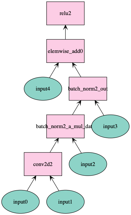
In the figure, conv2d2 is group_master, while relu2 is group_root; note the difference. Inputs coming from other subgraphs are replaced by input?.

Code Generation

Finally, based on the series of subgraph information (FuseEntry), we call TVM's codegen backend to generate actual operator code. This is mainly the following steps:

First traverse all subgraphs and call GraphLower() to compile them down to the final low level IR (i.e., HalideIR), mainly applying loop transformations to produce transformed code. Note that each OP corresponds to a series of LoweredFunc objects.
Then we need to generate a new computation graph. Note the difference between graph construction here and the previous step: previously we only built the structure of each subgraph to generate code for each fused subgraph, but the computation graph itself was not adjusted to the fused structure, so it cannot be executed yet. So in this step we need to adjust the computation graph into a fused structure with correct dependencies that can execute. The algorithm is straightforward: traverse the original computation graph in forward topological order, build a corresponding new Node for each subgraph, set its attributes, and correctly set connections between subgraphs, i.e., fill the Node.inputs vector.
Finally, call the compilation backend to compile all LoweredFuncs into executable binary code, and set it into the "module" attribute of Graph. At this point, the graph compilation pipeline is done; afterwards there are still runtime-related optimizations such as memory allocation, which are unrelated to graph compilation.

A schematic of a fused computation graph is shown below; the input label is removed to make node names clearer (Resnet-18):

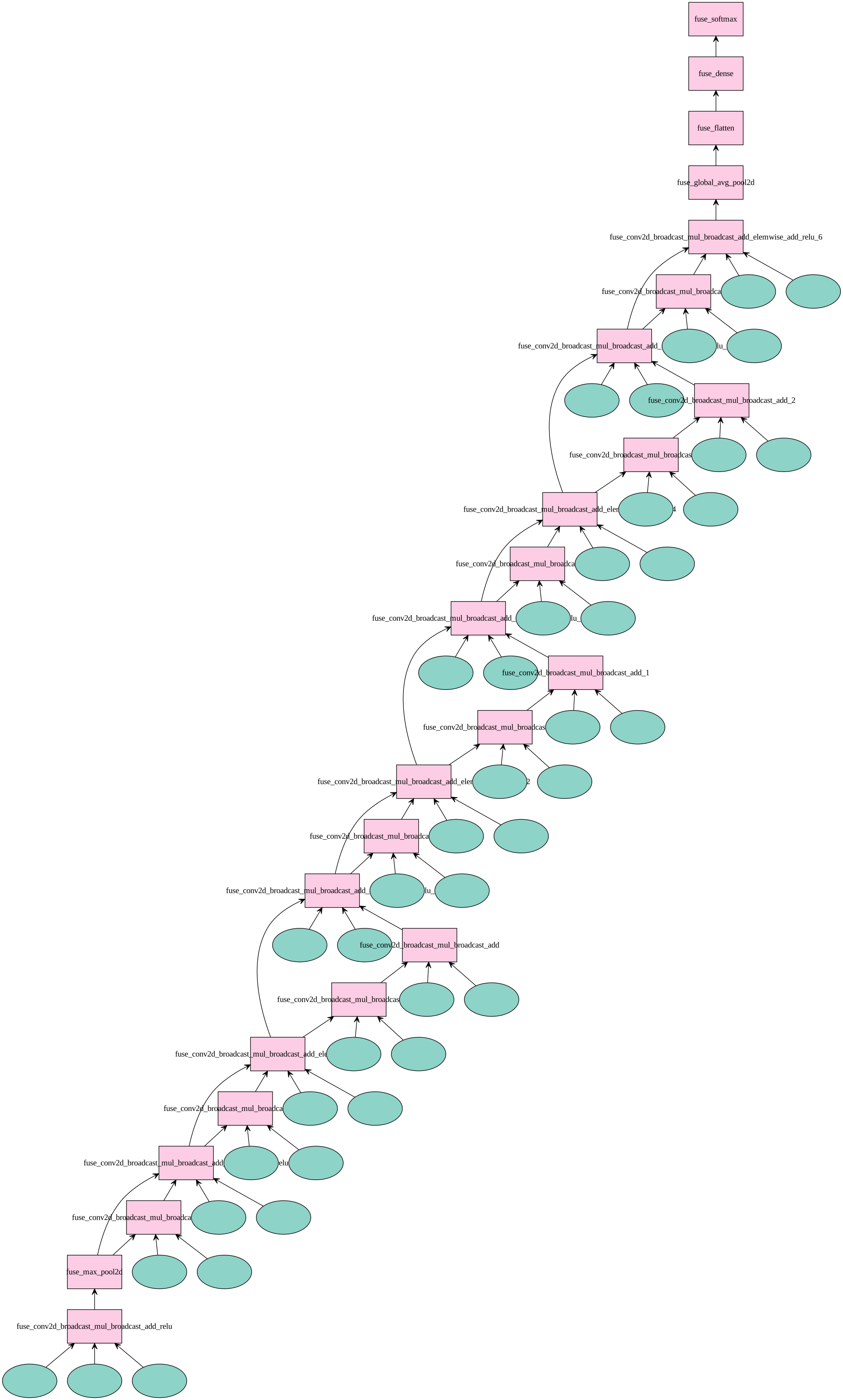
As you can see, although the fused computation graph still has crossing edges, it has completely become a serialized form.

Code Style & Complaints

In one sentence, TVM's overall style feels like writing C++ with Python instincts.
The Operator registration mechanism (Registry) uses a bit too much global state, and some optimization tricks seem not very meaningful; the macro API design is fairly nice though. While spreading operator registration across source files to register different attributes is a good idea, it cannot actually implement arbitrary overriding of already-registered attributes: this steps right into the pitfall where C++ has undefined initialization order of static variables across translation units—in practice, initialization runs in reverse link order.
Even though templates are everywhere, the code does not use static types well to constrain things; seeing the parameter strings inside Op::GetAttr<FGradient>() everywhere is unpleasant.
The computation graph optimization part adopts a structure of one pass per compilation unit; readability is so-so. The graph-building data structures look like they borrowed from LLVM; without specific benchmarks, let's assume a design like IndexedGraph provides some optimization benefits.
The Python interface and ctypes part is excellent, and the collaboration with NNVM_REGISTER_OP is very elegant, making C++-implemented operators automatically register into modules during import. It's just... a bit twisty to read.